Physically based Pathtracer

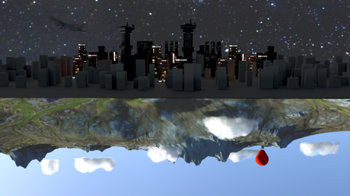
A physically based pathtracer built in C++ as part of ETH Zürich’s computer graphics course, extended with advanced rendering features including volumetric media, Disney BRDF, and low-discrepancy sampling. The renderer is based on Nori, a minimal pathtracer framework providing model loading, ray-triangle intersection, and BVH acceleration. During the homeworks I implemented features such as diffuse, specular and dielectic materials (with multiple importance sampling), and photon mapping. he final project was done in a group of two with my friend contributed environment map and many-light sampling.

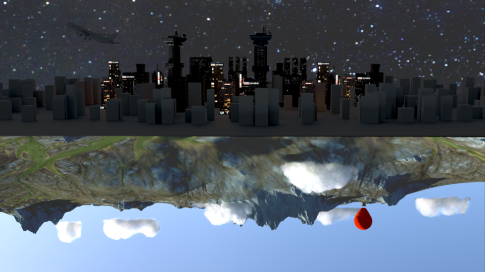Final renderer

I will now discuss the interesting features implemented by me.

Halton Sampling

#

We replace Uniform sampling with Halton sampling due to its low discrepancy. Halton sampling is done using Halton Sequences. For a sample we compute the n-th number (index) in the halton sequence of base k. For the next sample we use the next prime as base. To avoid correlation we pick a random index depending on the pixel position and permute the sequence of prime bases.

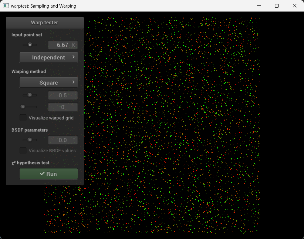
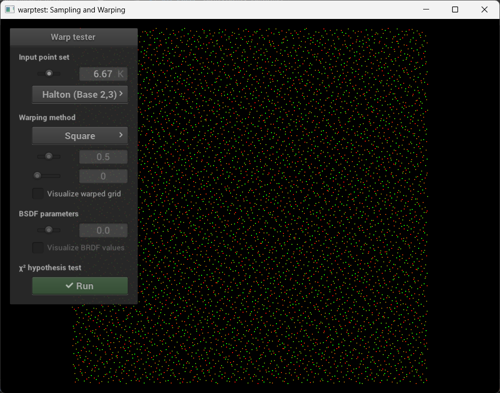
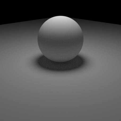
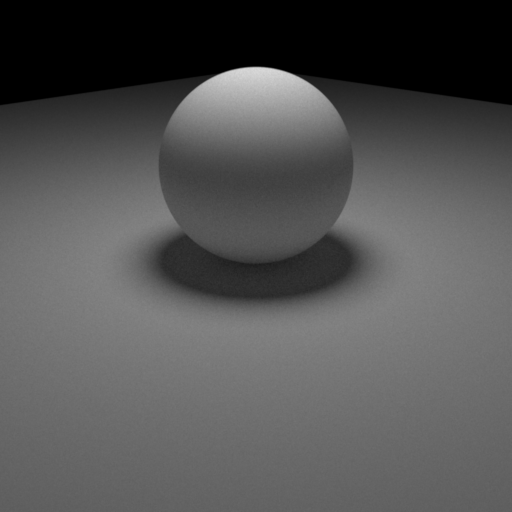
Uniform (top) compared to Halton sampling (bottom; base 2 and 3)

Here a comparison between uniform and halton sampling both with 16 sample per pixel (spp).

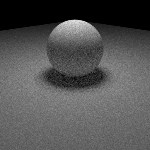
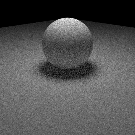
While Halton sampling is more expensive it still performs better when compared to uniform sampling using the same render time of 1.2 min. The Independent sampler used 1412 spp and Halton 1024.

Disney BRDF

#

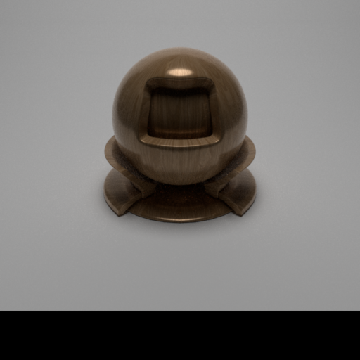
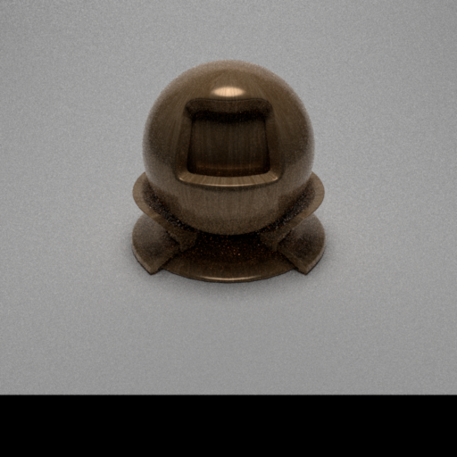
I implemented the Disney BRDF with the parameters: Roughness, Metallic, Anisotropic, Sheen, Sheen Tint. To check the correctness I compared my rendering with Mitsuba using a mesh from here. Anistropic materials needed consistent tangent frames so I implemented Computing Tangent Space Basis Vectors for an Arbitrary Mesh.

Also important to add was texture support for the materials.

Heterogeneous Participating Media

#

Heterogeneous participating media is rendered using delta tracking and supports isotropic and Henyey-Greenstein phase functions. The code uses nanovdb for loading the volume.

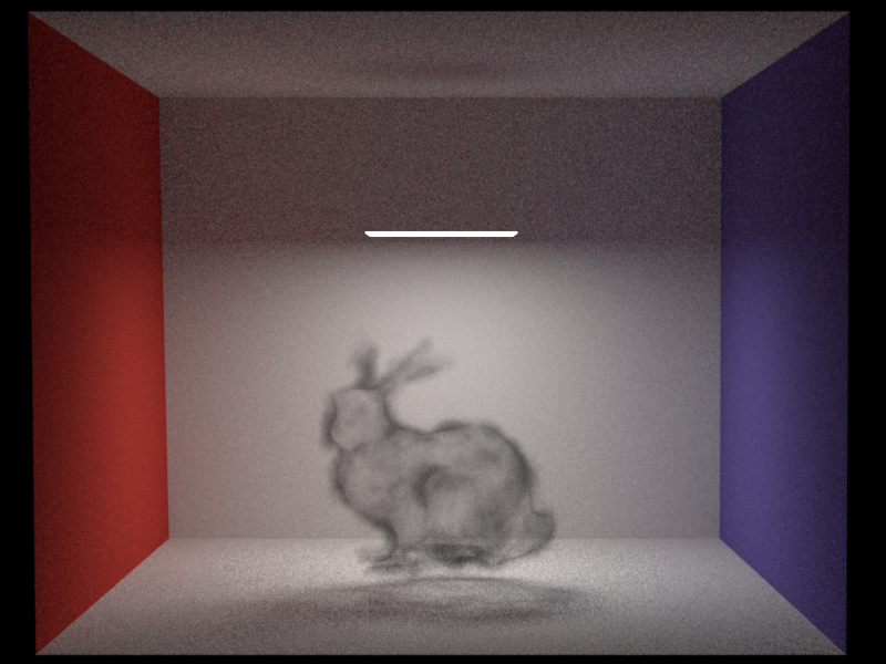
Volume with Henyey-Greenstein phase function (g = 0.8)